1.
Hydrological Cycle and Water Budget of a River
A typical hydrological cycle is shown in Figure 1.
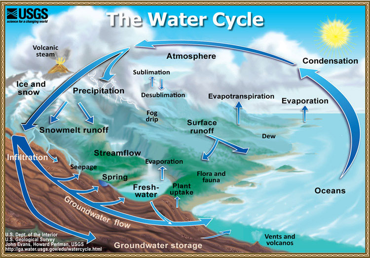
Source: https://water.usgs.gov/edu/graphics/watercyclesummary.jpg
The components of hydrological cycle (atmospheric, surface and ground waters) are intimately interlinked over spatial scales (from meters to thousands of kilometers) and temporal scales (from days to millions of years). The physical and chemical properties of water, render this substance to be an extraordinary biological, chemical and geological agent that made life possible on Earth.
The hydrological cycle is driven mostly by solar energy and to a minor extent by geothermal heat. The Earth’s erosional and geochemical cycles are due to water’s ability to do the mechanical work of erosion, chemically interact with rocks and minerals and transport the dissolved and suspended materials. Altogether, the hydrological, erosional and geochemical cycles constitute the vital cycles that sustain life [2].
According to the dictionary, a water budget is an accounting of all the water that flows into and out of a project area. This area can be a river, a wetland, a lake, or any other point of interest. Development can alter the natural supply of water and severely impact an area, especially if there are nearby ponds or wetlands.
A water balance equation can be used to describe the flow of water in and out of a system. The water budget equation would be expressed as follows:
P = E + Rsu + Rgw + ΔSu + ΔSo + Dh
where P is precipitation, R is runoff, Su is the surface water, Gw is the ground water, Δ represents the accumulation or change in storage and Dh is the diversion by humans.
There are many factors that affect waters budget and use. For example, local water budget factors include precipitation, temperature, vegetation, wind and the seasons.
The greatest factor controlling streamflow, by far, is the amount of precipitation that falls in the watershed as rain or snow. However, not all precipitation that falls in a watershed flows out, and a stream will often continue to flow where there is no direct runoff from recent precipitation.
When rain falls on dry ground, some of the water soaks in, or infiltrates the soil. Some water that infiltrates will remain in the shallow soil layer, where it will gradually move downhill, through the soil, and eventually enters the stream by seepage into the stream bank. Some of the water may infiltrate much deeper, recharging groundwater aquifers. Water may travel long distances or remain in storage for long periods before returning to the surface.
The amount of water that will soak in over the time depends on several characteristics of the watershed:
- Soil characteristics: Soils made mostly of clay and rocks absorb less water and at a slower rate than sandy soils. Soils absorbing less water results in more runoff overland into streams.
- Soil saturation: Like a wet sponge, soil already saturated from previous rainfall can't absorb much more ... thus more rainfall will become surface runoff
- Land cover: Some land covers have a great impact on infiltration and rainfall runoff. Surfaces made of asphalt, such as parking lots, roads and developments, act as a "fast lane" for rainfall - right into storm drains that drain directly into streams.
- Slope of the land: Water falling on steeply-sloped land runs off more quickly than water falling on flat land.
Evaporation: Water from rainfall returns to the atmosphere largely through evaporation. The amount of evaporation depends mostly on temperature, solar radiation, wind and atmospheric pressure.
Transpiration: The root systems of plants absorb water from the surrounding soil in various amounts. Most of this water moves through the plant and escapes into the atmosphere through the leaves. Transpiration is controlled by the same factors as evaporation, and by the characteristics and density of the vegetation. Vegetation slows runoff and allows water to seep into the ground.
Storage: Reservoirs store water and increase the amount of water that evaporates and infiltrates. The storage and release of water in reservoirs can have a significant effect on the streamflow patterns of the river below the dam.
Last term, Dh, represents the water use by people. The use of a stream might range from a few homeowners and businesses pumping small amounts of water to irrigate their lawns to large amounts of water withdrawals for irrigation, industries, mining, and to supply populations with drinking water.
No matter how different rivers are, however, all of them share some basic anatomy features. A tributary is a river that feeds into another river, rather than ending in a lake, pond, or ocean. If a river is large, there’s a good chance that much of its water comes from tributaries.
The beginning of a river is called its headwaters. Even if a river becomes big and powerful, its headwaters often don’t start out that way. Some headwaters are springs that come from under the ground. Others are marshy areas fed by mountain snow. A river’s headwaters can be huge, with thousands of small streams that flow together, or just a trickle from a lake or pond. What happens in the headwaters is very important to the health of the whole river, because anything that happens upstream affects everything downstream.
The shape of a river channel depends on how much water has been flowing in it for how long, over what kinds of soil or rock, and through what vegetation. There are many different kinds of river channels - some are wide and constantly changing, some crisscross like a braid, and others stay in one main channel between steep banks. The bends in a river called “meanders” are caused by the water taking away soil on the outside of a river bend and laying it down the inside of a river bend over time. Each kind of river channel has unique benefits to the environment.
The land next to the river is called the riverbank, and the streamside trees and other vegetation is sometimes called the “riparian zone.” This is an important, nutrient-rich area for wildlife, replenished by the river when it floods.
Floodplains are low, flat areas next to rivers, lakes and coastal waters that periodically flood when the water is high. The animals and plants that live in a floodplain often need floods to survive and reproduce. Healthy floodplains benefit communities by absorbing floodwaters that would otherwise rush downstream, threatening people and property.
The end of a river is its mouth, or delta. At a river’s delta, the land flattens out and the water loses speed, spreading into a fan shape. Usually this happens when the river meets an ocean, lake, or wetland. As the river slows and spreads out, it can no longer transport all of the sand and sediment it has picked up along its journey from the headwaters.
Wetlands are lands that are soaked with water from nearby lakes, rivers, oceans, or underground springs. Some wetlands stay soggy all year, while others dry out.
Flow refers to the water running in a river or stream. There are two important aspects to a river’s natural flow. First, there is the amount of water that flows in the river. Some rivers get enough water from their headwaters, tributaries, and rain to flow all year round. Others go from cold, raging rivers to small, warm streams as the snowpack runs out, or even stop flowing completely. A river’s natural ups and downs are called “pulses.”
The second component of natural flow is how water moves through a river’s channel. In a natural, wild river, the water runs freely. But in more developed or degraded rivers, dams and other structures can slow or stop a river’s flow [3].
To have a better idea about the water budget, two watersheds will be analyzed in this unit. Both watersheds have similar overall amount of precipitation, but they differ in terms of temperature/climate.
The two watersheds are Ohio River at Dam 53 near Grand Chain, Illinois (site identification # 03612500) and Missouri River at Hermann, Missouri (site identification # 06934500, according to United States Geological Survey gauging stations site inventory). The monthly and yearly data collected for both watersheds are from 1992 to 2004.
The annual average temperatures are 12.1
o
C for Ohio and 7.8
o
C for Missouri basin.
Although both watersheds enjoy similar amounts of precipitations, they have very different hydrology [4]. The Missouri river receives the highest volume of precipitation, approximately 724 km
3
per year, followed closely by Ohio river, receiving 642 km
3
per year. However, when compared to the surface area of each basin (522,500 square miles and 203,100 square miles, respectively), the amount of precipitation for the Missouri river is only 0.53 m per year, compared to 1.22 m/year for the Ohio.
Furthermore, in the Missouri, the majority (87.8 %) of the rainfall entering the basin is lost to evapotranspiration (636 km
3
per year) and therefore the Missouri has the lowest discharge contribution (only 88 km
3
per year).
By comparison, the Ohio river loses only 58% of its precipitation to evapotranspiration (371 km
3
/year), leading to the largest discharge of all US major basins (271 km
3
/year), even greater than upper Mississippi watershed (117 km
3
/year).
The relationship between the annual precipitation, annual discharge (D) and annual evapotranspiration (E), between the two watersheds is presented in the table below [4].
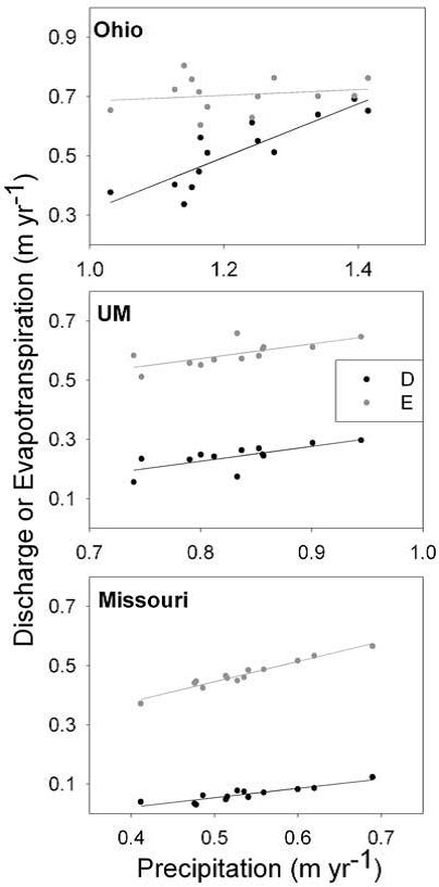
As the table suggests, any variation in precipitation is strongly correlated to a variation in discharge. The slope of precipitation versus discharge curves are 0.90 and 0.32, for the Ohio and Missouri, respectively. This indicates that a 10-cm interannual change in precipitation in the Ohio, leads to a 9.0-cm increase in discharge, while for the Missouri a 10-cm increase in precipitation only results in a 3.2-cm increase in discharge.
It is important to note, however, that because of the Missouri’s low discharge, the smaller increase in discharge can translate to a large percentage change in its annual discharge [4].
Hydrological Cycle Lesson Plan (two class periods)
Learning Objectives
Students will be able to:
- explain the water cycle of Earth
- define the terms associated with the water cycle
- explain the heat transfer processes associated with each component of the water cycle
Materials & Teacher-developed Resources
- Paper, pencils, textbooks, software
- Student handouts
- 500 mL jar
- a large dish
- heat lamp
- plastic wrap
- water
- rubber band
Learning Activities:
The teacher will review the states of matter.
Then, he reminds students the main components of water cycle: evaporation, condensation, precipitation and run-off, the thermal processes involved and phase changes for each component.
The teacher fills up the jar with 500 mL lukewarm water and pour it into the dish (“the lake”). Then, covers the dish with plastic wrap.
Place few ice cubes on top of the plastic wrap.
Turn on the heat lamp and place it in such way that the light shines down onto the “lake”. Set the model aside and wait for 20 minutes.
Ask students to complete their handouts and describe what they observe.
Ask students to explain why it was necessary to add water to the “lake” in this model.
Predict what would happen if water was not present.
Explain the role if ice cubes and heat lamp in this model and what would have happened if they were not present.
At the end, ask students to evaluate the model. Are there any stages of the water cycle not represented in this model? Explain.
Water Budget of a River Lesson Plan (one class period)
Learning Objectives
Students will be able to:
- demonstrate understanding of the principle of conservation of mass as it applies to a river and a watershed
- define the terms involved in the water budget equation
- perform computations using the water budget equation
Materials & Teacher-developed Resources
- Paper, pencils, textbooks, software, calculators
Learning Activities:
The teacher will review the students’ base understanding of the water cycle. Then, introduce and explain the terms of the water budget equation for a watershed. To simplify the equation, the teacher will explain that the water cycle of a watershed will be considered a closed system, where the storage water amount results as a difference between the input (precipitation) and output (evapotranspiration and runoff) amounts.
To simplify the computations, the teacher will specify that ground water flux and the diversion by humans are neglected.
Students will solve problems to estimate the annual runoff, given the total amount of precipitation and the loss due to evapotranspiration (both in cubic meters, centimeters or in terms of a daily rate for evapotranspiration).
2. Chemistry of Carbon in Freshwaters
Carbon is a highly mobile element that has the ability to change sides easily between inorganic and organic matter. Its cycle goes through atmosphere, biosphere, hydrosphere and lithosphere. Due to the fact that it can be found in many oxidation forms (oxidation number could vary from -4 to +4), carbon can be found in millions of compounds in gaseous, liquid or solid phases.
The cycle of carbon is usually thought of as four major reservoirs of carbon interconnected by pathways of exchange. The reservoirs are the atmosphere, the terrestrial biosphere (which usually includes freshwater systems and non-living organic material, such as soil carbon), the oceans (which includes dissolved inorganic carbon and living and non-living marine biota), and the sediments (which includes fossil fuels).
The Global Carbon Cycle
According to Sarmineto and Gruber [5], the organic carbon buried in sediments as coal, natural gas, and oil over hundreds of millions of years is being consumed as a result of human activities and returned to the atmosphere as carbon dioxide (CO
2
) on a time scale of a few centuries. The energy harvested from this transformation of fossil fuels supplies us with electricity, heat, transportation, and industrial power.
The clearing of forests for agricultural lands and the harvesting of wood, both of which remove carbon-bearing vegetation, have also added CO
2
to the atmosphere, in amounts equivalent to more than half of the fossil fuel source. The CO
2
added to the atmosphere because of man’s activities, and the way it is currently distributed within the land, air, and sea, is depicted in the carbon cycle diagram shown in figure 2.
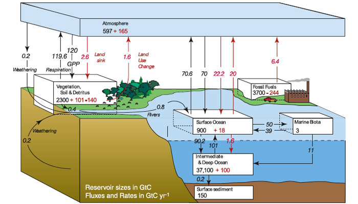
Source: https://www.learner.org/courses/envsci/visual/img_lrg/global_carbon_cycle.jpg
Because CO
2
is nonreactive in the atmosphere, it has a relatively long residence time there. However, its growth rate is presently less than half of what would be expected if all the CO
2
released by fossil-fuel burning and land-use change remained in the atmosphere. The growth rate is lower because the terrestrial biosphere (plants and soils) and the ocean are taking up a significant amount of anthropogenic CO
2
, that is, acting as “sinks” [5].
The ocean contains the largest active pool of carbon near the surface of the Earth, but the deep ocean part of this pool does not rapidly exchange carbon with the atmosphere.
The Carbon Cycle of the Inland Waters
The carbon absorbed by the land doesn’t necessarily stay there. Recent global studies suggest that more than half of that carbon every year ends up in inland waters, roughly 2.7 billion metric tons. Half of the carbon is respired and returned to the atmosphere as CO
2
. In general, because rivers and streams import CO
2
from soils and groundwater in their watershed, they emit substantially more CO
2
than lakes do [8].
Carbon dioxide is also produced by various microorganisms from fermentation and cellular respiration.
Most carbon of freshwaters occurs as equilibrium products of carbonic acid.
Carbonic acid is the most important weathering agent. The partial pressure of carbon dioxide (CO
2
) in an aqueous solution (a solution in which the solvent is water) dictates the path of a reaction that involves minerals containing carbonate (CO
3
) and silicate (SiO
4
) ions. The increase in carbon dioxide gas, either through respiration or increased burning of fossil fuels, can also have a large effect on alkalinity of those waters, because weathering is enhanced at the lower pH and calcium carbonate minerals present may dissolve and release alkali as follows [2]:
2[H
+
] + [CO
3
2-
] + CaCO
3 -----
>
Ca
2+
+ 2[HCO
3
-
]
In addition to the inorganic reactions, life processes extract CO
2
from water through the process of photosynthesis or add CO
2
when organic matter is consumed by respiration. Plants convert carbon dioxide to oxygen during photosynthesis, using both the carbon and the oxygen to produce carbohydrates. In addition, plants also release oxygen to the atmosphere, which is subsequently used for respiration by heterotrophic organisms, forming a cycle.
The carbon chemistry of rivers and lakes has been severely affected by human activities. The increase of erosion following deforestation and agriculture removes carbon from the biosphere into inland deposition centers, lakes and reservoirs and causes the organic carbon load of rivers to increase. Organic sewage and eroded soil carbon fuel respiration in rivers, thus increases the CO
2
pressure and diminishes the oxygen and nitrate loads in relation to the total organic content.
Nutrient release causes eutrophication of lakes and coastal seas, resulting in enhanced primary productivity and CO
2
sequestering. Loss of calcium carbonate (CaCO
3
) in upstream lakes causes increasing undersaturation of streams with respect to carbonate minerals.
By building dams and reservoirs, regulating the stream bed, diverting water for irrigation, and discharging agricultural, industrial and municipal waste into rivers and lakes humans have altered dramatically the hydrography and hydrochemistry of most fresh waters. These changes have their consequences with regard to the chemistry of carbon in rivers and lakes, as follows:
-
Deforestation and the spread of large-scale mechanized agriculture increases soil erosion and loss of humic soil-material to rivers.
-
Waste waters introduce unstable (fast decomposing) organic substances into lakes and streams, thus stimulating respiratory activity that raises the internal CO
2
pressure and acidifies the water while depriving it of its oxygen.
-
The leaching of nitrates from agriculture and the sewage inputs of ammonia, nitrite, nitrate and phosphate can cause vigorous phytoplankton blooms in lakes, reservoirs and coastal seas. The water becomes more alkaline and inorganic carbon is converted to organic carbon. The excess organic carbon is either buried in lake sediments or respired when washed out into free running rivers.
-
Altering the CO
2
pressure of a body of water by respiration and photosynthesis has an immediate effect on carbonate mineral saturation state. Acidified rivers can dissolve additional carbonate if more is available and lakes with algal blooms can precipitate excess carbonate as calcite (multiple forms / crystalline structures of calcium carbonate, CaCO
3
).
The distribution of CO
2
and pH in surface waters varies both seasonally and vertically in lakes in relation to loading from allochthonous sources, physical solutions, and with biotic inputs and consumption.
A smaller amount of carbon occurs in organic compounds as dissolved and particulate organic carbon and a small fraction occurs as carbon of living biota. The two components, dissolved organic carbon (DOC) and particulate organic carbon (POC) account for the total organic carbon (TOC) amount present in a stream or watershed.
Dissolved organic carbon (DOC) is defined as the organic matter that is able to pass through a filter that generally have a range in size between 0.7 and 0.22 µm. Dissolved organic carbon refers to a broad group of molecules that come from the breakdown of organic matter in a watershed. It consists of a variety of molecules that range in size and structure from simple acids and sugars to complex humic substances.
A common example of dissolved organic carbon comes from tea - as dissolved organic compounds emanate from tea leaves when they are introduced into water. Similarly, dissolved organic carbon from leaves and other organic matter lend a brown tinge to lake water, reducing water clarity. In many lakes and reservoirs, dissolved organic carbon and algae are the top two contributors to low water clarity. Water clarity is a huge feature that regulates a number of other characteristics of lakes and reservoirs, such as the depth to which photosynthesis occurs, the depth to which UV radiation penetrates, and heat budgets.
Indigenous dissolved organic carbon can enter a system through precipitation, leaching and decomposition. Highly productive wetlands can generate massive amounts of organic matter that enter lakes and watersheds primarily in dissolved form. Landscape parameters are strongly correlated with dissolved organic carbon, color and total organic carbon (TOC) in lakes and streams and include the drainage ratio, slope of the terrain, water residence time and percentage of the watershed covered by wetlands.
Dissolved organic carbon is of interest to ecologists as it can affect physical, chemical, and biological properties of freshwater systems. Through attenuation of solar radiation, dissolved organic carbon can provide UV-B (short ultraviolet wave radiation) protection to aquatic microflora and fauna and depress primary productivity in lakes.
Reductions in dissolved organic carbon concentrations can increase lake transparency. The fulvic and humic acids of dissolved organic matter can influence the acid-base chemistry of freshwaters, affecting the cycling of metals such as copper, mercury, and aluminum and thus influencing the amount of trace metals found in aquatic organisms. Dissolved organic carbon can also support bacterial secondary production, influence the availability of some forms of phosphorus to phytoplankton and alter sedimentation rates.
Landscape parameters are strongly correlated with dissolved organic carbon, color, and total organic carbon in lakes and streams, and include the drainage ratio, slope, water residence time and percentage of the watershed covered by wetlands. Wetlands and wetland soils are often the source of much dissolved organic carbon input to lakes and streams, even though they may occupy only a small percentage of the catchment area.
Particulate organic carbon (POC) is defined as the large organic matter that is removed from a sample by filtration. This organic matter comes mostly from detrital terrestrial plant and soil material. The transport of particulate organic carbon in streams and rivers has proven to be a significant component of local and global carbon budgets.
Recent studies have shown that approximately 180 million metric tons of terrestrial particulate organic carbon is exported to the world’s oceans, while dissolved organic carbon exports are estimated around 250 million metric tons [6].
Generally speaking, the flux of particulate organic carbon in a watershed is estimated as a product between the discharge and the concentration of carbon in transported sediments. This concentration is largely determined by the types of soils and vegetation within each basin and the extent of interaction between runoff and soil [1].
For example, on the lower Hudson River basin (watershed area of 13,670 km
2
) for a sediment flux of 20.8 tons/km
2
per year, the particulate organic carbon flux was 1.64 tons carbon/km
2
per year. By comparison, on the upper Hudson River basin (watershed area of 10,110 km
2
) for a sediment flux of 8.3 tons/km
2
per year, the particulate organic carbon flux was only 0.6 tons carbon/km
2
per year. Both watersheds are characterized by a mixed land use (forested, agricultural, pasture and urban) [7].
It has long been recognized that across system, variation in the flux of carbon from watersheds is strongly correlated with precipitation. Within a watershed, annual variation in precipitation is also a driver of the annual export of carbon.
However, there is a sharp contrast in the response of dissolved organic matter and particulate organic matter export to discharge rate of a stream. Concentrations of dissolved substances are relatively little affected by the flow rates, whereas particulate organic matter concentrations are directly and exponentially related to the system discharge.
As a consequence, the bulk of particulate organic matter is moved during storms. The output of dissolved substances is therefore related to annual output of water, while the removal of particulate matter is more of a stochastic process, strongly related to the occurrence of random storms [2].
It is also highly likely that the change of the way land is used alters the relationship between precipitation and carbon export. Wetland loss has decreased the export of dissolved organic carbon from areas of the United States by as much as 20-30%. Agricultural practices have augmented the amount of bicarbonate and particulate organic carbon available for export to streams while cities and suburbs have greatly altered stream hydrology and presumably carbon export [3].
Determining the pH of a Substance Lesson Plan (one class period)
Learning Objectives
Students will be able to:
- determine if a solution is acidic, basic or neutral
- learn about the pH and pOH as measures of acidity and alkalinity, respectively
- determine the pH of few different samples of water, coming from a river, pond, or a lake
Materials & Teacher-developed Resources
- Paper, pencils, student handouts
- Aprons
- Safety goggles
- Spoons
- Test tube racks
- 1 Glass stirring rod
- pH (litmus) paper
- Paper towels
- 10 ml graduate cylinders
- 100 ml graduate cylinders
- Distilled water
- Eye Droppers
- Small or medium test tubes
- Ammonia
- Apple juice
- Baking soda solution
- Coffee
- Corn syrup
- Laundry detergent
- Lemon juice
- Milk
- Tomato juice
- Water Samples (from a river, a pond and a lake)
Learning Activities:
The teacher will start the lesson by discussing properties of acids and bases. Acids are usually sour; bases usually bitter. Identify the potential harm acids and bases can create. Discuss critical safety procedures like “Do Not Ingest” and “Do Not Mix”.
Then ask: How does an indicator help us figure out what is an acid, base or neutral? Introduce acidity/alkalinity of substances using an indicator to determine their differences and discuss safety precautions in handling of each. The teacher will explain that pH is the symbol for the degree of acidity or alkalinity (base) of a substance. pH also refers to the potential of hydrogen in a substance.
Then, the teacher introduces the pH scale
0 1 2 3 4 5 6 7 8 9 10 11 12 13 14
Acid (H3O+) Neutral Alkaline (Base, OH-)
As the hydronium ion H3O+ concentration increases the acid concentration increases. For example: a substance with a pH reading of 1 is a stronger acid than a substance with a pH reading of 6. Likewise, as the hydroxide ion (OH-) concentration increases, the alkalinity increases. For example: a chemical with a pH reading of 12 is a stronger base than a chemical with a pH reading of 8.5. Substances with a pH reading of 7 are neutral. The reaction of an acid with a base produces salt and water. In neutralization, the properties of the acid and base are lost as two neutral substances water and a salt are formed.
Then ask students to place a strip of litmus paper into each box of pH worksheet (see attachment).
-
Using the eye droppers, put few drops of each chemical into the test tubes
-
Dip the stirring rod into first test tube
-
Record the color of the indicator strip in the data table
-
Clean up the stirring rod after each use
-
Hold the indicator strip next to each color key. Determine which color matches the strip
-
Record the pH that corresponds to the color in the data table
-
Repeat steps 2-6 for each substance
Based on their findings, students classify the given chemical substances into acids, bases or neutrals.
The teacher will direct the students to write for ten minutes in their journals summarizing the lab and all procedures used in this lesson.
The Carbon Cycle Lesson Plans (three class periods)
Learning Objectives
Students will be able to:
- explore the human factors that contribute to the rise of carbon dioxide into the atmosphere
- determine how different inputs to the carbon cycle might affect the concentrations of the greenhouse gas CO2
Materials & Teacher-developed Resources
Student handouts, pencils, textbooks, Carbon Cycle Interactive Lab Simulation software
Learning Activities:
Under the teacher’s supervision, students will run the simulation to the year of 2110 with the default settings. Using their Data Table, ask students to record the total carbon levels in each "sink" (terrestrial plants, soil, oil and gas, coal, surface ocean, and deep ocean) for the years 2040, 2060, 2080 and 2110.
Using the data collected from the model, answer the following questions while thinking about how the model mimics real-life conditions:
- If only one half of the flora in the world existed in 2110 (perhaps due to deforestation), what do you predict the atmospheric carbon level would be?
- How would you change the simulation to reflect this?
- What is the relationship between increased carbon in the ocean and increased carbon in the soil?
- How else might carbon be transferred to soil?
- Using the data generated by the simulation, determine the mathematical relationship between the percentage increase in fossil fuel consumption and the increase in atmospheric carbon. Is the relationship linear?
To find out where all the carbon really goes, students will run the simulation again, one decade at a time. Ask them to record the total amount of carbon in the atmosphere (the number in the sky) and other carbon sinks (terrestrial plants, soil, surface ocean, and deep ocean), as carbon moves through the system. Finally, students will be required to answer the following questions:
- What is the relationship between an increase in fossil fuel consumption and increased carbon in terrestrial plants?
- How might this change flora populations?
- What impact could twenty years at this level of consumption have on flora?
- What is the relationship between an increase in total carbon concentration (the smokestack) and increased carbon in the ocean surface?
- How might this change marine life populations?
- What impact could fifty years at this level of emissions have on marine fauna? On marine flora?
- In addition to circulating through the carbon cycle, where else might excess carbon be found?
- In fifty years, where would you be most likely to see excess carbon?
- Which areas are most highly (and quickly) affected by an increase in carbon emissions (and increase in fossil fuel consumption)?
- How would these effects manifest themselves?
-What are the dangers/benefits to these areas?
Role of Water Treatment Plants Lesson Plan (one class period)
Learning Objectives
Students will be able to:
- explain how does a water treatment plant work
- describe what turbidity is and how it influences the water treatment processes
- explain the basic steps of water purification in such plant
Materials & Teacher-developed Resources
Student handouts, pencils, textbooks, Secchi tube turbidity meter, different water samples water treatment simulation software
Learning Activities:
The teacher will start the lesson by asking students “What are the main indicators of water quality?” (Answer: Turbidity and bacterial tests). Students will record their answers. Then, ask them to brainstorm a list of ways that water can be polluted (factory chemicals, fertilizers, pesticides, animal, human and industrial waste).
Next, the teacher introduces the concept of turbidity (cloudiness of water) and explain how it is measured (in nephelometric turbidity units, NTU) using the water samples and Secchi tube turbidity meter.
Students will practice measuring the turbidity of each water sample, noting the nephelometric turbidity units, NTU, for each sample.
They will explain also how the engineers have contributed to the improvement of quality of life in industrialized countries by providing safe drinking water to their populations.
The teacher will introduce the main components and explain the role of each step of a typical large-scale drinking water treatment plant:
-
Primary (gross) filtration, or settling basin, where water is filtered through screens that remove fish, leaves and trash
-
Coagulation and flocculation, where alum (hydrated potassium aluminium sulfate) is added to form sticky flocs, followed by sedimentation to remove the flocs (large groups of particles) from water
-
Secondary (fine) filtration, where the water trickles down through sand and gravel to remove algae, bacteria and some chemicals still present in water
-
Chlorination, where chlorine is added to destroy the remaining bacteria, viruses and pathogens
-
Aeration, where air is forced through the water to remove gases that produce undesired odors or tastes
-
Additional treatment station, where sodium and lime may be used, to soften the hard water. Some plants add fluoride, which helps prevent tooth decay
Students will discuss the water distribution systems and answer the final two questions:
- How do the water distribution systems affect the environment and the world?
- What are some of the small-scale water treatment systems engineers design and install?