Lesson 1: Evaluating and Developing Graphical Representations of Quadratics
Overview
Students will begin their exploration of quadratic functions by evaluating functions and developing graphical representations of these functions. Evaluating the functions to create a table of values, students will graph multiple quadratic functions so they can familiarize themselves with the basic appearance of a parabolic graph. This is a 45-minute lesson.
Objectives
Students will be able to…
|
1.
|
evaluate a quadratic function using function notation, and
|
|
2.
|
graph a quadratic function by plotting a set of ordered pairs.
|
Warm-Up with Teacher Notes
Students will complete the warm-up handout, which reviews function notation and how to evaluate functions in function notation. The warm-up is meant to help scaffold the rest of the lesson, which will rely heavily on evaluating functions. Students should need no more than 5 minutes to complete this assignment. When the class is done, ask students to quickly go around the room and compare answers. Are there any discrepancies? Allow students to explain the problems to one another. You can assume that some students did not square -1 properly and therefore made a mistake in #3. Have a student review #3 on the board if a lot of the students made this mistake.
Prompt:
f(x), said "f of
x," is how we express the value of the function when
x
is a given value. This notation is known as function notation
.f(x) =
is equivalent to
y =
. For example,
f(x) = 3x + 2
, find
f(5)
In other words, what is the value of
y
when
x = 5
f(5) = 3(5) + 2 = 15 + 2 = 17
Let
f(x) = x
2
+ 3x - 2.
. Determine the values of…
1.
f (2)
2.
f (0)
3.
f (-1)
Mini-Lesson
Give a mini-lesson in which you review the definition of a quadratic function. How does a quadratic function differ from a linear function? What might a quadratic function look like? Ask the students to develop a hypothesis about what a quadratic function would look like. Students will check their hypotheses in the next activity.
Graphing Quadratic Functions Activity
This is a small group activity. Divide the class into groups of two or three. Each group will be assigned one of three prompts. Ask students to evaluate the function over a defined interval

and to create a t-table of values. Students should be familiar at this point with t-tables and how to plot points from a t-table. Step 1 for each group requires the same skills, but offers a slightly different prompt so groups can make comparisons later in the activity.
Each group should be given an oversized piece of chart paper on which to write their function, their t-table, and to draw a graph. Students should follow the prompts on the handout for setting up their graph. Step 2 is the same for all groups.
Once students have completed their graphs, have them display their graphs next to one another on the wall. Students will complete a gallery walk to compare and contrast the overall appearance of the graphs. What do quadratic functions look like? What was similar about each of the graphs? How did they differ? Students will then share their observations with the class during an all-class discussion.
Graphing Quadratic Functions Activity Prompt 1
Hang gliders are small aerial crafts that people usually fly for recreation. You are a photographer at a hang gliding show. You were instructed to take a photo every 10 seconds in order to capture the movement of the hang glider's dive. The dive is modeled by the equation
f(x)=(1/100)x
2
- (25/2)x +30
, where
x
represents the time since the dive started and
f (x)
represents the height of the hang glider.
|
1.
|
Determine the hang glider's location every 10 seconds for the first 100 seconds of the dive by evaluating
f (0), f (10), f (20), f (30), … , f (90), f (100)
. Record these values in the t-table below.
|

Graphing Quadratic Functions Activity Prompt 2
Catapults were medieval weapons designed to launch an object, usually for destructive purposes. You are designing a catapult that launches a boulder along a trajectory given by the equation
f(x) = - (1/10)x
2
+ x + 6
, where
x
represents time and
f (x)
represents the height of the projectile.
|
1.
|
Determine the boulder's position every 2 seconds for the first 14 seconds after it's been shot by evaluating f (0), f (2), f (4), … , f (12), f (14). Record these values in the t-table below.
|

Graphing Quadratic Functions Activity Prompt 3
You were instructed to design an apparatus for a skate park in a nearby neighborhood. A skateboarder's position on the apparatus is modeled by the equation
f(x) = 2(x-2)
2
, where x represents seconds and f (x) represents the skateboarders height from the ground.
|
1.
|
Determine the skateboarder's position on the apparatus for the first 10 seconds by evaluating
f (0), f (1), f (2), f (3), … , f (9), f (10).
Record these values in the t-table below.
|

Graphing Quadratic Functions Activity Part 2 (same for all groups)
|
2.
|
On a large sheet of graph paper, create a graph using the data from the table. Be creative in your representation of the scenario.
|
|
3.
|
You will complete a gallery walk to compare and contrast several different quadratic functions. Divide a sheet of paper up into three columns: similarities, differences, and other observations as seen below. Record any observations you have about the graphs of each function. How are the graphs similar? How do they differ? Are there any interesting features?
|

Homework
You launch a catapult that has a trajectory given by the equation
f(x) = -(1/2)x
2
+ 3x + 5
where
x
represents the number of seconds since the projectile was launched and
f (x)
represents the height of the projectile.
1. Complete the following t-table by evaluating the equation given above.

2. Create a graph that depicts the trajectory of the catapult by plotting the ordered pairs given in the table in question 1.
3. Use the graph to answer the following questions.
|
a.
|
What is the initial launch height of the projectile?
|
|
b.
|
How high can the catapult launch something?
|
|
c.
|
How many seconds does it take the projectile to reach the highest point along its trajectory?
|
|
d.
|
Along what interval is the projectile's height decreasing?
|
|
e.
|
Describe what happens to the projectile during the interval
7 < x < 8.
|
|
f.
|
Is
f (9)
feasible? Explain why or why not within the context of this problem.
|
Lesson 2: Analyzing Graphical Representations of Quadratic Functions
Overview
Students will begin learning key terminology and familiarizing themselves with the key components of parabolic curves: the vertex, absolute maximum/minimum,
y-;
intercept, x-intercept(s), and increasing and decreasing intervals along the curve.
Objectives
Students will be able to…
|
1.
|
identify the vertex and line of symmetry of a parabola, its concavity, the regions in which the function is increasing and decreasing; and
|
|
2.
|
determine the domain and range of a parabola.
|
Warm-Up
|
1.
|
Graph the function
f(x) = (x + 1)
2
−3
on a sheet of graph paper by evaluating the function over the interval
|
-

|
2.
|
Identify the
highest
point along the curve.
|
|
3.
|
Identify the
lowest
point along the curve.
|
Class Notes and Discussion
The prior activity will lead into a discussion on what quadratic functions look like graphically. Class notes should review definitions of parabolas, increasing and decreasing intervals, extrema, domain, range, the line of symmetry, x- and y-intercepts and concavity. Review several examples until students are able to identify each of these components on a graph. Students will practice identifying these components within context in the next activity.
Flashback to Lesson 1
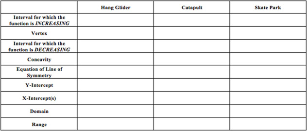
Examine the posters (Hang Glider, Catapult, and Skate Park) each group made during Lesson 1. Analyze each poster, and record the following information in the table below.
Homework
You launch a catapult that has a trajectory given by the equation
f(x) = (−1/2)x
2
+ 2x + 5
where
x
represents the number of seconds since the projectile was launched and
f (x)
represents the height of the projectile.
|
1.
|
Graph the function on a sheet of graph paper by evaluating it over the interval
|
-

-
|
2.
|
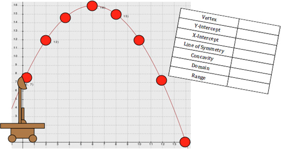
Identify each component in the graph. Then, record it in the table below.
|
Lesson 3: Modeling Quadratic Functions
Overview
Students will learn how to perform a quadratic regression in order to determine the equation of a quadratic function given a set of data points. Students will begin interpreting the significance of the vertex, the intercepts, and increasing/decreasing intervals.
Objectives
Students will be able to…
|
1.
|
input data into a graphing calculator;
|
|
2.
|
perform various regressions to assess what type of model fits a set of data the best and to determine an equation that approximates a model of the data; and
|
|
3.
|
use a quadratic regression model in order to interpolate/extrapolate desired data points.
|
Warm-Up
A catapult was launched and the projectile followed the path seen in the graph. Use the graph to complete the table below. Each axis is scaled by 1.

Graphing Calculator Mini-Lesson
Students will be given a set of notes on how to perform a regression on a set of data. Students will learn about the coefficient of determination and what r
2
values indicate about the fit of the model to the data. Walk students through a couple examples of how to perform a regression by looking at several data sets for practice. Data sets can be found on the Math Tidbits website. It is important to look at non-quadratic models so students gain a richer understanding of how to determine what type of model fits the data best.
Regression Models and Developing a Best-Fitting Curve Activity
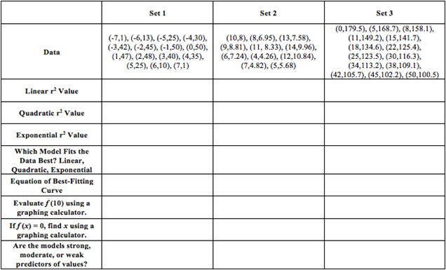
Perform linear, quadratic, and exponential regressions for the following sets of data. Determine which model fits the data best by examining the coefficient of determination. Finally, record the equation of each model.
Lesson 4: Exploring the Effects of Altering Coefficients
Overview
This lesson serves as the capstone project to this unit. Students will explore how adjusting various components of the catapult affect the equation of a quadratic function. Students will attempt to tie these changes directly to the coefficients of the quadratic model
y = ax
2
+ bx + c.
In the end, students will make predictions about what kind of adjustments they can perform to the catapult in order to alter the equation to meet a desired theoretical outcome.
Warm-Up
Show a clip from Top Gear Series 4 Episode 4. This clip introduces students to a car catapult and is a good illustrator of the parabolic trajectory of a catapult launch. Use this time to discuss with students what engineers must consider when designing an apparatus like a catapult. Ask students to consider how parabolas can be manipulated. Transition from this discussion into the Unit Project.
Unit Project
Students should be divided into groups of approximately three to four. Each group will be provided a catapult. Depending upon the amount of time available, the teacher can assign each group to perform each experiment, or can ask each group to complete only one experiment. For a shorter span of time, assign each group to complete only one experiment and then have students share their results. Once all groups have recorded all the data, students will be able to complete the analysis.
Provide a basic demonstration to the class that shows how to use the catapult, how to adjust its various components, and review the location of the three points being collected. Data from the demonstration should be recorded on the board and will serve as the data for the control group. All data collected by groups after altering a component to the catapult will be compared directly to this control data.
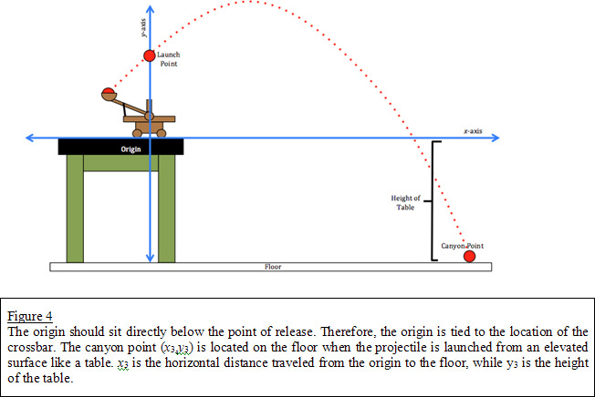
The launch point is the point of release. This point is located at
(0,y
1
)
, as seen in Figure 1, where y
1
should be the height of the catapult when the arm is vertical. The ground point is
(x
2
,0). x
2
is the horizontal distance of where the projectile hits the ground. The third point is labeled the canyon point since students will move the catapult to an elevated surface for the final launch. Explain to the students that whatever surface the catapult sits on serves as the x-axis. Although the floor may initially serve as the x-axis, once the catapult has been repositioned to a table, for example, the table becomes the new x-axis. When the catapult is repositioned onto an elevated surface, the graph's window is changed to include the third and fourth quadrants, or the region in which
y < 0
.
Experimental Procedure
To determine a model for the projectile, it is necessary to collect several data points. For this project, you will perform numerous trials and perform a quadratic regression to determine an equation that approximates the parabolic trajectory of the projectile.
To begin, copy the initial information for all the catapults from those used in the control group in the demonstration. This information should be recorded below. Every group should begin with the same initial information except in ONE (1) instance. The teacher will instruct each group to either vary the arm length, the angle of release, or the number of times the rubber band is twisted. It is essential that students only vary one of these components, otherwise they will not be able to attribute any changes in flight directly to the change in the apparatus.
Have the alterations written down before class begins to make it easier to assign what alterations each group will perform. One group will shorten the arm length, while another will lengthen it. One group should decrease the angle of release, while another increases it. Finally, one group should reduce the number of twists, while another increases the number of twists of the rubber band.
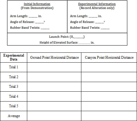
Follow these steps to measure the vertical and horizontal distance the catapult can launch a projectile. Let x represent the horizontal distance the projectile travels. Let y represent the vertical distance the projectile travels.
|
1.
|
Set the catapult on the floor. Launch the projectile and measure the horizontal distance to where the projectile hits the floor. Call this point the Ground Point. Perform 5 trials. Record the data in the table above.
|
|
2.
|
Set the catapult on a flat, elevated surface (every group should use the same elevated surface for consistency). Measure the vertical distance from the base of the catapult to the floor. Launch the projectile and measure the horizontal distance to where the projectile hits the floor. Call this point the Canyon Point. Perform 5 trials. Record the data in the table above.
|
|
3.
|
Determine the average horizontal distance of the Ground and Canyon points.
|
|
4.
|
Input the three points (Launch, Ground, Canyon), as seen in Figure 2, into the STATS menu of your graphing calculator. Perform a quadratic regression to determine an equation for the best-fitting curve of the projectile's trajectory.
|
Have the two groups that altered the arm length compare their three equations (their two plus the control equation from the demonstration). Have the two groups that altered the angle of release compare their two equations with the control equation. Finally, have the two groups that altered the torsion of the rubber band compare their two equations with the control equation. Are there significant changes in the equation, or did only certain coefficients change? It may be necessary to point out to the students that some changes to the coefficients may be insignificant while others are quite large.
Reflection and Conclusion
|
1.
|
Record the three equations below:
|

|
2.
|
Highlight any coefficients that are significantly different. Is there one coefficient that was affected more than the others?
|
|
3.
|
Write a conclusion that explains how altering a specific component of the catapult will affect the trajectory equation of the projectile.
|
Groups should present their results to the class. If the experiments went well, the group that changed the arm length should have equations that are nearly identical with the exception of c, the y-intercept. The angle of release group should notice that a, the leading coefficient, is significantly different. Students should be able to make a connection to the fact that changing the angle of release caused the parabola to widen or narrow, which they know by now is caused by the leading coefficient either being greater than or less than 1, respectively. Finally, the torsion group should have relatively similar
a-
and
c-
values as the angle of release and the initial launch height did not change. The
b
coefficient, however, should differ for each equation.
Refer to the following prompt and your conclusions from earlier in the lesson to answer the questions below. Students will need to consider manipulations of the catapult apart from those that they were assigned in their original groups.
A catapult launches with a trajectory given by the equation
f(x) = − 1/4x
2
+ 2x + 5
.
|
1.
|
Identify two manipulations to the equation that would result in the catapult being able to launch further.
|
|
2.
|
Identify what adjustments to the catapult would result in the desired manipulations to the equation you mentioned in question 1.
|
|
3.
|
If the arm length and angle of release are decreased, explain what will happen to the trajectory of the projectile. What type of changes do you expect to occur to the coefficients of the equation? Explain your reasoning.
|
The last component of this activity is to have students use what they know about manipulating the catapult to alter their equations in order to hit specified targets. Provide three targets around the room, each of varying distance from the catapults. Ask the students to evaluate the control equation to see if adjustments are necessary. If
y = 0
, then the catapult is positioned correctly. Position one target so no adjustments are needed. Position the other two so students must adjust their catapults to hit the targets. Students should know what type of adjustments will increase or decrease the distance the catapult launches the projectile.
Algebra 1 Alternative
Alternatively to the Algebra 2 approach to the project, students can make alterations to just one component of the catapult and test to see whether altering arm length, for example, yields a linear or non-linear change in horizontal distance thrown. This slight alteration introduces students to modeling without necessarily going to in depth into quadratics, making it a more algebra 1 friendly project.