Experimentation and Data Collection
The scientific method is commonly used in science classrooms and has served as a guide for how to enter into scientific inquiry. The key steps include:
|
1.
|
Asking a question;
|
|
2.
|
Researching;
|
|
3.
|
Constructing a hypothesis;
|
|
4.
|
Testing the hypothesis through experimentation;
|
|
5.
|
Analyzing data;
|
|
6.
|
Drawing conclusions; and
|
|
7.
|
Communicating your results.
|
In this unit, students are provided a question: How do adjustments to various components (arm length, angle of release, and spring torsion) of a catapult affect the trajectory of a projectile? Students will have a chance to examine the catapults, informally assess the various components, and perform basic research before creating a hypothesis about how altering the arm length, angle of release, and spring torsion affect the trajectory of the projectile.
In science, a hypothesis is commonly referred to as an educated guess; that is, a statement that suggests that there is insufficient evidence to declare the statement always true. Hypotheses are established as a guide to the experiment. They provide focus and purpose. Students research possible contributing factors in an effort to predict the outcome of their experiment. Creating a hypothesis also encourages students to think deeply about how to approach the question, ultimately hitting the first standard for mathematical practice: make sense and persevere. Predicting the outcome of an experiment, even if incorrect, helps students make sense of the parameters.
Experimentation is often overlooked as a mathematical practice and immediately skipped for data analysis. Performing an experiment, however, gives a different insight into the interpretation of data as it gives students ownership of the material. An experiment is a scientific procedure used to test the validity of a hypothesis. The key component to an experiment is the procedure. When performing an experiment, it is necessary to have an explicit procedure. The goal of an experiment is not to stumble upon random results, but rather to establish a procedure that can be duplicated to further support the initial results.
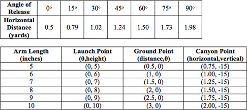
Perhaps the simplest way to record data is using a table. In this experiment, students will make use of a t-table; that is, a multiple column table that relates the independent variable (the manipulative) with the dependent variable(s) (the experimental result). T-tables can be recorded horizontally or vertically. Two examples can be seen below:

One way to minimize poor data collection is to hold as many variables constant as possible. During any test scenario, it is crucial that only one variable change at a time, so the effects can be directly attributed to those changes. If two variables change, how does the student know which change caused the result? For example: a student launches a projectile and it travels a horizontal distance of five yards. The student then adjusts the arm length and the angle of release and the same projectile travels a horizontal distance of eight yards. Can the three yard increase in horizontal distance be contributed to the change in arm length, the change in the angle of release, or both? How much did each change affect the outcome? Holding all but one variable constant allows the experimenter to limit the factors that may have caused change (remember, there may be variables that change that the experimenter does not realize are being changed). If the student only changes the arm length and the projectile travels six yards, then the student can assume the one yard increase was caused directly by a change in the arm length.
The last item to consider when performing an experiment is to perform multiple trials. Increasing the number of trials reduces the effects of error within the experiment. Just because a catapult launches five yards once, doesn't mean that it will consistently launch five yards. Multiple trials help account for outliers and other data that could skew the results. The law of large numbers states that the average of a large number of trials in an experiment will approximate the expected value. Therefore, the more trials performed, the more likely the experiment will yield results that reflect the true value of the experiment (in this case, the horizontal distance traveled by the projectile). A generally accepted rule of high school science states that three trials are appropriate when performing an experiment. Performing three trials allows you to collect several data points without taking too much time to repeat the experiment.
Analysis of Data, Regression Modeling and the TI-84 Plus
Data analysis will mostly utilize regression modeling on the TI-84 Plus. Once students have collected their data, they will enter it into a table and create a scatter plot.
3
To enter data into a table:
|
·
|
Push [STAT], [1].
|
|
·
|
Enter the independent variable data into L1 and the dependent variable data into L2, pressing [ENTER] after each entry.
|
|
·
|
Press [2
nd
], [MODE] to QUIT and return to the home screen.
|
To create a scatter plot:
|
·
|
Press [2
nd
], [Y=] to access the STAT PLOT editor.
|
|
·
|
Press [ENTER] to edit Plot1.
|
|
·
|
Press [ENTER] to turn On Plot1.
|
|
·
|
Scroll down and highlight the scatter plot graph type (first option in the first row). Press [ENTER] to select the scatter plot type.
|
|
·
|
Scroll down and make sure Xlist: is set to L1 and Ylist: is set to L2. To input L1, press [2
nd
], [1]. To input L2, press [2
nd
], [2].
|
|
·
|
Press [GRAPH] to display the scatter plot (you may need to adjust the window). To fit the data to a specific window, press [WINDOW] and enter appropriate values for the extrema and the intervals. For a quick fit, press [ZOOM], [9] to perform a ZoomStat.
|
To perform a regression:
|
·
|
Press [STAT], scroll right to display the CALC menu.
|
|
·
|
Scroll to one of the regression models and press [ENTER] to select the regression type you want to perform. You will now be on the HOME screen.
|
|
·
|
Press [2
nd
] [1] [,] [2
nd
] [2] to indicate which lists the data is saved in. Press [,] [VARS]. Scroll right to bring up the Y-VARS menu. Press [1] [1] to store your regression in the Y= menu as Y
1
. Press [ENTER].
|
If the above procedure is followed correctly, the calculator will display the results of the regression, including the equation for the selected model that best-fits the data and the coefficient of determination. The coefficient of determination is also known as the r
2
value and indicates how well interpolated and extrapolated data fit the regression model. The coefficient of determination is such that
0 ≤ r
2
≤ 1
. Two variables with a high r
2
value
(r
2
> 0.8)
are said to show a high degree of correlation, meaning you can us e one variable to predict the value of the other. Two variables with a low
r
2
value (r
2
< 0.5)
are said to show a low degree of correlation, meaning one variable is not a good predictor of the value of the second. A moderate
r
2
value may or may not indicate that the regression model is a close fit for making predictions. Note that there is not an agreed upon number scale for how well the r
2
value indicates a degree of correlation between variables.
Interpolation is a process used to predict an intermediate value of the dependent variable; that is, a value that lies somewhere between the highest and lowest values of the data. Extrapolation is a process used to predict values outside the given data by extending the regression curve.
Quadratic Functions and Their Key Features
Quadratic functions in standard form are defined as
f(x) = ax
2
+ bx + c
, where
a
,
b
and
c
are real numbers and a ≠ 0.
4
The parent function
f(x) = x
2
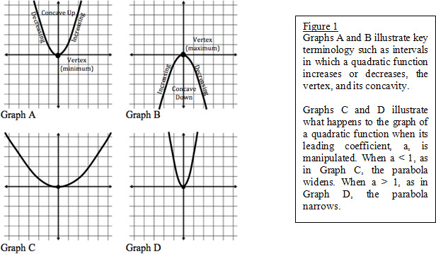
can be seen in Graph A below. The shape of the graph is known as a parabolic curve, or a parabola. Note that parabolas are composed of an increasing interval (as x increases, y increases) and a decreasing interval (as x increases, y decreases). The vertex of a parabola is the point at which the curve transitions from increasing to decreasing or vice versa. The vertex is known as the minimum (Graph A) or as the maximum (Graph B). A parabola is concave up if it opens upward; that is, its end behavior is increasing as in Graph A. A parabola is concave down if it opens downward; that is, its end behavior is decreasing as in Graph B.

The coefficients
a
,
b
, and
c
reveal a lot of information about the shape of a parabola. The leading coefficient,
a
, indicates the narrowness of the parabola along with the concavity. If
0 < |a| < 1
, then the parabola will appear wider, as in Graph C.
If
|a| > 1
, then the parabola will appear narrower, as in Graph D. These changes are known as dilations and occur because the quadratic term,
x
2
, is being made smaller or larger, respectively, when it is multiplied by a. A parabola is concave up if
a > 0
and concave down if
a < 0.
The constant term,
c
, is known as the y-intercept; that is, the point where the curve intersects the
y-
axis. This is easily derived. All points along the y-axis have an
x
-coordinate of
0
. Thus, the y-intercept can be calculated
f (0) = a(0)
2
+ b(0) + c = c
.
The leading coefficient,
a
, and the linear coefficient,
b
, can be used to calculate the line of symmetry. All parabolic curves have a line of symmetry given by the formula
x= -b/2a
. The line of symmetry acts like a mirror and marks the horizontal distance at which the parabolic curve switches from increasing to decreasing or vice versa. As such, the line of symmetry can be used to determine the maximum or minimum y-value of the curve. Once the vertical line of symmetry is found, the vertical max or min can be found by evaluating the function
f( -b/2a)
For example, determine the vertex of the quadratic function
f(x) = 2x
2
+ 4x−5
. Therefore, x= - 4/(2(2))= - 4/4= - 1. The minimum value occurs when
x = -1 f(-1) = 2(-1)
2
+ 4 (-1) - 5 = 2 - 4 - 5 = -7.
Thus, the vertex, or minimum point, of the parabola is
(-1, -7).
Finally, all three coefficients can be used to calculate the x-intercept(s) (also known as the solution(s) to the function) using the quadratic formula, which states that the x-coordinate can be calculated as,

Note that the formula includes a ±, suggesting two possible solutions. Because quadratics have one turn at the vertex, the curve can intersect the x-axis in a maximum of two locations, though it may not intersect at all (as is the case when there are complex solutions to the quadratic formula). It is also possible for the quadratic to only have one solution if the vertex lies on the
x-;
axis.
The number and type of solutions to a quadratic function can be determined by examining the discriminant,
b
2
- 4ac
. If the discriminant
> 0
, then there will be two real solutions. If the discriminant
= 0
, there is only one real solution. And if the discriminant is
< 0
, then there are two complex solutions.
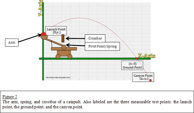
In this unit, students will launch projectiles that have a parabolic trajectory where the vertex does not lie on the x-axis. As such, the equations to the quadratic functions will have negative leading coefficients that result in curves that are concave down (as seen in the figure below). Consequently, this unit will focus solely on quadratic functions with two real solutions. Take note that one of the solutions will be extraneous as the domain is restricted to the first and fourth quadrants of the coordinate plane. Students will study other variations of quadratic functions in later units.
