Hydrology
The hydrological cycle is simply how water circulates around the globe. The watershed is the boundary, or area of land, in which all of the water that comes into this area drains to a single waterway. Also known as a water basin, a watershed can be thought of as funnel- any water that enters the watershed that remains as runoff will drain into a single point such as a stream, lake, or ocean. The main source of water entering the watershed is through precipitation, but any water that enters a system, including snowmelt, water from a sprinkler system, or even a bottle of water dumped out on the ground, will end up at the same place. Watersheds are naturally divided into regions by what are known as drainage divides, and where the precipitation falls in relation to the drainage divide will dictate where the water will ultimately end up.
1
For example, McNamee Peak, in Colorado, sits on the verge of three watersheds- the Arkansas River Watershed, the Colorado River Watershed, and Platte River Watershed. Because all of these watersheds drain into vastly different places, precipitation that falls within just a few feet of each other could potentially end up thousands of miles away.
2
Watersheds vary in size, which are classified by order. All watershed systems begin with first order streams, which are spring fed- no other bodies of water feed into a first order stream. As the streams flow downhill, two first order streams converge to form a second order stream, two second order streams converge to form a third order stream, and so on. Streams that are first through third order are considered headwater streams, and 80% of all waterways are headwater streams, by length. Streams of order four through six are considered medium size streams, and streams of order seven and above are classified as rivers- for example, the Ohio River is an eighth order stream, while the largest river in the world, the Amazon, is considered a 12
th
order stream. Eventually these rivers will feed back into the ocean– for example the Ohio River will eventually join with the Mississippi River (a tenth order stream), which will ultimately flow south into the Gulf of Mexico, while the aforementioned Amazon River flows from west to east into the Atlantic Ocean. Not every stream leads to the ocean, however - some feed into landlocked lakes or wetlands.
3
The Water Cycle
Water moves through the watershed through the hydrologic system, which is defined as, "the process by which water moves from the atmosphere to land surfaces precipitation, infiltrating the subsurface or flowing along land surface to the oceans, and eventually returning to the atmosphere by evaporation".
4
All water is in one of four places- the oceans, the atmosphere, the land surface, and the subsurface, and water is constantly cycling through the atmosphere at varying rates - some water that falls as precipitation may evaporate in a matter of hours, while some water may stay in the ocean or frozen in ice for thousands of years.
However, fresh water, which humans and other living organisms rely on, is a limited resource – of the 332.5 million cubic miles of water on the planet, only about 0.01% is in circulation and available for human consumption. Of the rest of the water, over 96% is saline, and of the remaining less than 4%, over 68% is locked up in ice and glaciers, and 30% of freshwater is in the ground. That leaves about 1/150
th
of a percent of water in fresh-water sources on the surface, such as rivers and lakes, which are the surfaces which humans use the most.
5
Water Budgets
The water budget is an accounting of the water stored within and water exchanged among the watershed. The water within the watershed is constantly in motion, and the water budget, or accounting for the water within the system, can be defined simply as the input of water to the system must be equal to the output of water leaving the system, plus or minus the change in storage. This can be related to a financial budget- the amount of money that you can cumulatively spend and/or put into savings must be equal to the amount of money that is put into your bank account to begin with. For the same reason that we track our financial budgets to make sure that we do not overspend and are using our financial resources wisely, it is important to track watershed budgets so that we can better manage our water resources.
Mathematically, the watershed budget can be written as
𝑃=𝐸+𝑅
𝑆𝑢
+𝑅
𝐺𝑤
+𝐷
𝑆𝑢
+𝐷
𝑆𝑜
+𝐷
𝐺𝑤
+𝐷𝐻
where P is precipitation, E is evapotranspiration, R
Su
is surface water runoff, R
Gw
is groundwater runoff, D
Su
is the change in surface water, D
So
change in soil water, D
Gw
is the change in groundwater and DH is the diversion of water by humans. Each of these terms are defined below.
6
Precipitation
Precipitation is water that is released from clouds, in the form of rain, freezing rain, sleet, snow, or hail, and it is the component of the hydrologic cycle in which water is released from the atmosphere. Precipitation most often falls in the form of rain. For context, one inch of rain falling on one acre of land is equivalent to 27,154 gallons of water.
In this unit, the unit of measure for water is kilometers cubed. One kilometer cubed of water (or a cube of water that is 1km on all sides) is equivalent to 264,172,052,400 gallons.
Precipitation varies widely across the globe- in some places, such as Georgia, it rains fairly evenly per month, averaging 40-50 inches per year. In more tropical regions, places may receive more rain, but only during certain “monsoon” seasons which are marked by long periods of intense rainfall.
7
Surface Runoff
Water that runs downhill over the surface of the land after precipitation becomes surface runoff. Proportionally, averaged over the whole globe about one-third of the water that enters the watershed through precipitation becomes surface water – the other two thirds is evaporated, transpired, or is absorbed by the ground. This amount can vary greatly from watershed to watershed depending on the overall climate. This surface runoff will eventually run into rivers and back out into the oceans, completing the water cycle. How surface water flows is largely dependent on not only the amount of rainfall, but also the physical geology of the land.
Scientists in environmental agencies such as the United States Geological Survey measure the volume of water that flows through a river or stream over time. This volume of water is known as discharge. Typically, discharge is calculated by taking the area of a cross section of a stream and multiplying it by velocity of the stream at that cross section. Since the area of a cross section of the river can be calculated by the depth of the river multiplied by the width, the general formula for calculating discharge is
discharge=width*depth*velocity
Scientists measure the velocity by placing gauges in streams which collect the necessary measurements. The United States Geological Survey collects data at 15- to 60- minute intervals from various sites in streams and rivers across the country, which is compiled into what are known as hydrographs.
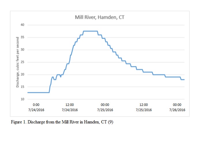
Hydrographs represent the streamflow in a river over time. The streamflow is constantly fluctuating, even on an hourly basis, but the main factor which alters streamflow is precipitation. Storm hydrographs are particularly telling about a watershed because even the influence of precipitation is dependent on the river itself. During a storm, large rivers, which have a larger surface area, will only result in a small increase of streamflow, while a small river could see an increase of 100 times its baseline streamflow. By analyzing a hydrograph along with precipitation data, scientists can determine how precipitation affects a specific watershed, which helps in the preparation and prediction of flooding of the surrounding land.
However, precipitation is not the only factor which influences the constant change in streamflow in a watershed. Other factors could include evaporation from soil and surface water, transpiration by vegetation, ground water discharge from aquifers, ground-water recharge from surface-water, and various human-induced factors, among others.
8
Figure 1 shows a hydrograph created for a local river which shows the daily discharge. The graph was made using data collected by the United States Geological Survey at the Mill River in Hamden, Connecticut, which was made available on the USGS website.
Evapotranspiration
Evapotranspiration is the combination of the water that is taken out of the system from both evaporation and transpiration. Evaporation is the process in which water is transformed from a liquid to a gas - evaporation drives the water cycle. Water can evaporate from surface water, such as streams, rivers, or lakes, and also directly from the soil. Transpiration, meanwhile, is the evaporation of water from the leaves of plants. Plants absorb water from the soil and some of the excess water is released through stomates in the leaves by through transpiration. While transpiration is an invisible and difficult to measure, it is not negligible and must be accounted for - an acre of corn gives off about 3,000-4,000 gallons of water each day through transpiration, and a large oak tree can transpire 40,000 gallons per year. Overall, studies have shown that 90% of evaporation comes from surface water such as lakes, rivers, and the ocean, while 10% of evaporation occurs as transpiration.
10
Groundwater Runoff
Runoff that does not stay on the surface of the watershed is absorbed by the land. The ground can be thought of as a giant sponge, which soaks up the water, which occupies the spaces between the soil and the rock particles. If the water infiltrates far enough to meet the water table, it can be carried out towards streams, the ocean, or deeper in the ground. When the water-bearing rock transmits water to wells and springs, it is known as an aquifer. This water can be accessed by wells drilled below the water table into the aquifer, and water can be pumped out for human consumption. While precipitation replenishes the aquifer over time, the rate of recharge is not the same for all aquifers, and over pumping of an aquifer too quickly can cause a well to run dry. Depending on how permeable and porous the subsurface rocks in the area are, the water can move quickly through the ground, or be sunk into deep aquifers where it can be trapped for thousands of years. Because these large aquifers take hundreds of years to accumulate water, they are negligible in the watershed equation, but are nonetheless important resources of water for humans.
11
In the United States, we rely on groundwater for over half of our needs, and because we are using the water at a faster rate than it can be replaced, many of these aquifers are being drawn down. These aquifers are not a renewable resource, and continued over-reliance on these water sources could cause water shortages in the future.
For example, California’s recent drought, which lasted over five years, led to an increase in dependence on groundwater, suggesting that 60% of California’s water usage came from groundwater. As the aquifers are being drained, the water table is dropping- in the Central Valley, wells that used to be 500 feet down must be drilled down to 1,000 feet or more.
Similarly, the Colorado River Basin is losing water as well- a satellite study has shown that the Colorado River Basin lost 15.6 cubic miles of water from 2004 to 2013. This is occurring all over the country- in the Chicago-Milwaukee area, residents have been relying on groundwater as their sole source of drinking water since 1864, which has resulted in groundwater levels being lowered by as much as 900 feet.
12
Storage
Watersheds are transient systems, and storage levels of water on the surface, in the soil, and in the ground vary seasonally. For example, in a temperate climate, the amount of surface water may spike significantly in the spring months due to melting snow, but may reach a low point during the summer due to increased evaporation. Water is also stored in groundwater, such as the aquifers mentioned above, and in surface water, such as lakes and reservoirs.
13
Reservoirs are often created by humans by damming rivers or lakes to create pools of water which can be controlled and diverted based on the demand of the community.
Diversion by Humans
Humans divert water for their own needs, such as by dams and reservoirs, including drinking water, agriculture, and recreation, and over 80 percent of the water we consume comes from surface sources such as lakes, rivers and streams. In California alone, there are over 25, 000 places that water in rivers are diverted for human consumption. The ways that humans divert water can often have negative environmental impacts - for example, dams can cause numerous environmental issues such as preventing fish migration, upstream flooding, delta starvation, and changes to the ecosystem.
14
However, when scientists look at water budgets over the course of years, the change in storage balances itself out over time and becomes negligible, except for the period of time when a new reservoir fills. When looked at from a geological timescale, even the diversion of water becomes insignificant, and the balance of water can be defined in terms of the inputs and the outputs to the system. Thus when interested in just annual time scales the water budget can be simplified to:
Precipitation = Discharge + Evapotranspiration
where discharge is a combination of surface water and groundwater runoff.
Because evapotranspiration is difficult to measure directly, scientists can rearrange the formula to:
Precipitation – Discharge = Evapotranspiration
to determine the amount of evapotranspiration in a watershed, using measures of precipitation and discharge.
6
Because the watershed has a basic equation which represents the input and output of water through the system, it conceptually segues nicely into Algebra and provides a foothold into the mathematics that students will be learning about this unit.
Graphing Points and Discussion of Independent versus Dependent Variables
Two related points are expressed on a Cartesian plane. The input, often known as the x variable, is plotted on the horizontal axis, and the output, often referred to as the y variable, is represented on the vertical axis.
In real world contexts, the input and the output are often referred to as the independent variable and the dependent variable, respectively. Independent variables are variables which are constant, and not affected by anything else in the problem. Dependent variables, however, are directly related to the independent variable- the dependent variable changes in direct response to the change in the independent variable. For example, time and temperature are classic examples of independent variables, while distance traveled or evaporation are possible examples of related dependent variables.
In scientific contexts, the independent variable is often referred to as the “controlled” variable, or what is changed by the person performing an experiment, and the dependent variable is what is observed as a direct result of that change. For example, if I increase the water pressure in a garden hose, more water will come out of the hose in a given amount of time. If I decrease the water pressure in the garden hose, the amount of water that comes out of the hose will slow down to a trickle. Therefore, what I can control in this situation- the water pressure of the garden hose, is the independent variable and what I observe –the volume of water coming out of the garden hose, is the dependent variable. This provides another context for students to conceptualize independent versus dependent variables.
Additionally, students should understand the nature of the relationship between the independent and dependent variables. Students should understand while the independent variable always affects the dependent variable, but the converse is not true. As in the preceding example, the water pressure in the garden hose is what is changing the volume of water emerging from the spout. However the converse of this situation is not true; the volume of water emerging from the spout is not driving the water pressure – the water pressure is clearly driving the volume of water.
Understanding Slope and Linear Relationships
When the relationship between independent and dependent variables is constant, this is known as a linear relationship. For example, consider a car driving down the highway on cruise control- students can easily calculate that at 55 miles per hour, after one hour the car will have traveled 55 miles, after two hours the car will have travelled 110 miles, after three miles the car will have travelled 165 miles, and so on with no variation. Students should be able to recognize that this relationship is linear- the rate of change between each point is constant. If graphed, this relationship will form a straight line.
The rate of change between each point is known as the slope. Mathematically, the slope is calculated as the change in the y-values over the change in x-values, but conceptually students should know slope as the rate of change. For example, in the highway example, the rate of change in the position of the car is the velocity, or speed of the car. As the velocity of the speed increases, the distance the car traveled relative to the amount of time spent driving will increase, and similarly as the velocity decreases, the distance the car travels relative to the amount of time spent driving will decrease.
Graphically, if a line is increasing as the graph moves from left to right, the slope is said to be positive. If the line is decreasing as the graph moves from left to right, the slope is said to be negative. If the line is flat, or horizontal, as the graph moves from left to right, the slope is said to be zero.
Slope is commonly represented by the letter m in equations, and to find slope, students should calculate the change in y over the change in x. As an equation, this is represented as
m=Δy/Δx=y
2
‐y
1
/x
2
‐x
1
Where (x
1
, y
1
) and (x
2
, y
2
) are any two points on the line.
Graphing Lines
Additionally, students should be able to recognize, write, explain, and graph equations which model linear relationships. Specifically, students should be familiar with the slope-intercept form of a line, represented by the equation y = mx + b. In this equation, m represents the slope of the line and b represents the y-intercept, or where the graph crosses the y-axis. Students should also understand this occurs when the x-value of the graph is equal to zero.
A simplified equation which might represent the graph of precipitation versus discharge in a watershed might be y=3/10 x ‐ 10, where x represents the amount of precipitation in the system and y represents the amount of discharge at the given level of precipitation. Students should recognize the role that slope plays in this equation, and be able to articulate that compared to a line with an equation of y=7/10 x ‐ 10, a much higher percentage of the precipitation is becoming discharge in the second equation versus in the first equation.
However, data rarely works out so neatly in the real world. While clean, rounded numbers make it easier to focus on the conceptual skills, once students demonstrate the foundational skills, students can move on to more authentic real-world scenario.
Real world Mathematics: Scatter Plots and the Line of Best Fit Using Watershed Hydrology
Consider the following table from the Mississippi River Watershed from 1992-2004:
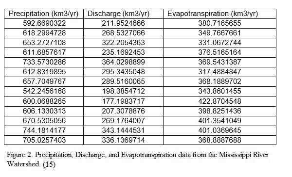
First, students should be able to create a scatterplot of the data by graphing each point on the Cartesian plane, and recognize that there is not one straight line that could neatly connect those points. At this point, students should distinguish between scatter plots that show a linear relationship and those where the relationship is not linear. However, they can recognize patterns in the data, and once students recognize the pattern that the data is trending linearly, a line of best fit can be created using graphing calculator or technology to create a line of best fit.
Using a graphing calculator, the line of best fit for precipitation versus discharge is y = 0.9012x – 0.5857 .
For comparison, it is also valuable to graph precipitation vs evapotranspiration for the same data set. If you graph precipitation versus exapotranspiration, the linear regression is y = 0.0988x – 0.5857. If you also graph the precipitation vs evapotranspiration, the slope of evapotranspiration (percentage of precipitation that evapotranspirates) + the slope of the discharge (percentage of water that becomes discharge) equals approximately one. This is logical, as water that does not evapotranspirates will become discharge, and vice versa.
Checking for Accuracy: the Correlation Coefficient and the Coefficient of Determination
Now that students have created a line of best fit, it is important for students to be able to analyze their line and see how well their linear regression accurately represents the data. There are two values that students should consider- the correlation coefficient and the coefficient of determination.
The first question students should consider is if the data is actually trending linearly.
In order to test whether the linear regression is truly a line of best fit, students should examine the correlation coefficient, also known as the r-value. The correlation coefficient measures the strength and the direction of the linear relationship between two variables. The r value always lies in-between positive one and negative one. The closer the r- value is to one, the stronger the correlation between the variables and the line. In general, a correlation over 0.8 is considered strong, while a correlation of less than 0.5 is considered weak. If the correlation is strong, then the linear function is a good model for the data set. If the correlation is weak, the data set may be better modeled by a different function (such as exponential or quadratic, for example). The plus and minus signs indicate direction – if the graph is increasing from left to right there will be positive correlation, but if the graph is decreasing from left to right there will be negative correlation. If the r-value is exactly one, that means that all of the points lie perfectly on a line. In the Mississippi River watershed, with calculations the r value is 0.87, which indicates a strong correlation.
The second question students should consider how well the regression represents the data set
.
In order to tell if the regression line accurately represents the data, students should consult the coefficient of determination, or the r
2
value. The coefficient of determination gives the proportion of the variance of one variable that is predictable by the other variable, which helps us determine how well the linear regression fits the data. If the linear regression is a good fit, it can be used as a model to predict values not explicitly included in the data set. However, if the line is a poor model, it will give an inaccurate estimation for the data if it is used as a model.
In the example above, the r
2
value is 0.76. This means that 76% of the data is explained by the relationship between x (precipitation) and y (discharge), but the other 24% of the variation remains unexplained.
Calculator Skills
It is vital that students have the necessary calculator skills to create and analyze linear regressions. Since calculators are most likely to be used on standardized tests, instructions to create scatterplots and linear regressions are included below. However, students may also create scatterplots and linear regressions by hand, through a different graphing calculator, or using a computer program, such as Microsoft Excel.
The steps to create a linear regression on a TI-84+ are as follows:
A. First, it is important to make sure that you have the correct settings enabled on your calculator:
-
Press [Stat], [5] (for “SetUpEditor”), and then [Enter]. This enables your list editor, where you will store your data used to create your scatter plot.
-
Press [2
nd
] and then [0] to bring up the catalog. Scroll down using the pointer keys until you reach “DiagnosticOn”. Press [Enter] twice. It is worth noting that in the catalog, alpha lock is automatically enabled. You may press [x
‐1
] to immediately jump down to the “D” section of the catalog.Turning Diagnostics on will tell you the r value, or the correlation of coefficient, and r
2
, or the coefficient of determination, when you calculate your linear regression.
-
Press [2
nd
] and then [Y = ] to bring up the stat plot menu. Press [Enter] to select Plot 1. Using the arrow keys, select “on” to turn on the stat plot and make sure that the XList is set to L1 and the YList is set to L2. This means that the x-values for the scatterplot will be pulled from list one and the y values will be pulled from the corresponding values in list 2. This step will allow you to view your scatterplot in the graphing window.
-
Press [2
nd
] and then [mode] to return to the main screen
B. Next, you can create a scatterplot.
-
Press [Stat] and then [Enter] to select the first choice on the menu screen, “Edit”
-
If there is any values written under L1 or L2 already, clear them out by pressing the [Del] key repeatedly. To clear the lists quickly, from the main screen you may also press [Stat], [4] to select “ClrList”, and then [2
nd
], [1],[,],[2], [Enter] to clear lists one and two.
-
Underneath the column for L1, list all of the x – coordinates, pressing the [Enter] key between each value to move to the next line.
-
Underneath the column for L2, list all of the y-coordinates, pressing the [Enter] key between each value to move to the next line. Ensure that the y-values are entered in the same order as the x-values, and that the corresponding x and y values of the coordinate are listed directly across from each other on the table.
-
When all of the data has been entered, you may press [graph] to view your scatterplot.
-
If the viewing window is not ideal to view the scatterplot fully, you may press [Zoom] and then [9] for the “ZoomStat” function, which will automatically select an appropriate window for your scatterplot.
C. Lastly, you can also calculate and graph the linear regression.
-
Press [Stat], and use the arrow keys to select the “Calc” menu. From there, you may either select [4] or [8], depending if you would like your linear regression to be in the form “ax + b” or “a + bx”, respectively.
-
Make sure that the XList is set to list one and the YList is set to list two. Use the arrow keys to move down to the option “Store RegEq”.This option will let you store the linear regression directly to the graphing window. To do this press [Vars], use the right arrow key to select “Y-Vars”, and then press [1] to select “function”. Press [1] again to select Y1.
-
Lastly, press the [enter] key twice to calculate the linear regression.
The screen will show you your linear regression, your correlation coefficient (r-value), and your coefficient of determination (r squared value). If you press [Y = ], you will see that your linear regression has already been entered into the graphing screen, and you may press [Graph] to view the graph of your scatterplot with the linear regression on top of it.
For comparison, it is also valuable to graph precipitation vs evapotranspiration for the same data set. If you would like to view this on the same window as the first graph, repeat all of the above steps, except enter the evapotranspiration values under L3. There is no need to re-enter the precipitation values, as they are still listed under List one. Repeat all of the preceding steps with the following changes:
A. Setting up your graphing calculator
-
You may skip steps A1 and A2, but under step A3, enable “Plot 2”, so you may graph the second set of data. Under Xlist, make sure that it is still set to L1, but next to YList, change the list to L3 by pressing the [2
nd
] key followed by [3]. Also, change the mark to a different symbol so that you can tell your two scatter plots apart.
-
Press [Y =], and then use the down arrow key to move to Y2. Then, press the left arrow key twice so that the “\” is selected. Press [Enter] to change the style of the line so that you can easily tell it apart from your first line.
B. Creating the scatterplot
-
In step B4, enter only your y-coordinates (remember, your x-coordinates are still listed under L1) under the L3 column.
C. Calculating the linear regression.
-
In step C3, Make sure that the XList is set to L1 and the YList is set to L3. To change the Y list from the default, simply press [2
nd
] followed by [3]. Use the arrow keys to move down to the option “Store RegEq”.This option will let you store the linear regression directly to the graphing window. To do this press [Vars], use the right arrow key to select “Y-Vars”, and then press [1] to select “function”. This time, press [2] to select Y2.